Learn image processing by seeing, coding, and experimenting
Study each concept with a visual example, compare Python and MATLAB commands, then log in to process your own images in the lab.
Laboratory Case Studies
Real-time results from DIP-Lab across all 12 image processing and medical imaging modules.
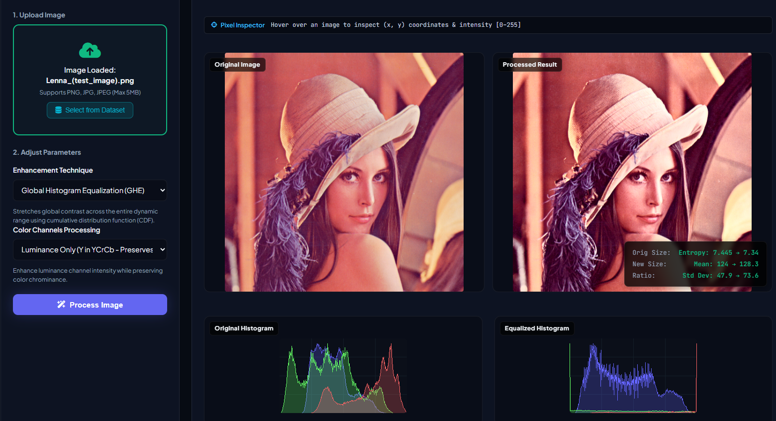
Image Processing Modules
Select a module to study its mathematical formulation and run real-time experiments in the lab.
Histogram Equalization
Enhance the global contrast of images by redistributing intensity frequencies evenly across the histogram.
import cv2
import numpy as np

# Grayscale Histogram Equalization
equalized_gray = cv2.equalizeHist(gray_img)

# Color Histogram Equalization (YCrCb)
ycrcb = cv2.cvtColor(color_img, cv2.COLOR_BGR2YCrCb)
ycrcb[:, :, 0] = cv2.equalizeHist(ycrcb[:, :, 0])
equalized_color = cv2.cvtColor(ycrcb, cv2.COLOR_YCrCb2BGR)
% Grayscale Histogram Equalization
equalized_gray = histeq(gray_img);
% Color Histogram Equalization (L*a*b*)
lab = rgb2lab(color_img);
lab(:,:,1) = histeq(lab(:,:,1)/100)*100;
equalized_color = lab2rgb(lab);Color Space Conversion
Convert images between different color models (BGR, Grayscale, and HSI) with side-by-side components.
import cv2
import numpy as np

# BGR to Grayscale
gray = cv2.cvtColor(img, cv2.COLOR_BGR2GRAY)

# Grayscale to JET pseudocolor
jet = cv2.applyColorMap(gray, cv2.COLORMAP_JET)

# BGR to HSI model conversion
img_f = img.astype(np.float32) / 255.0
b, g, r = cv2.split(img_f)
i = (r + g + b) / 3.0
num = 0.5 * ((r-g) + (r-b))
den = np.sqrt((r-g)**2 + (r-b)*(g-b)) + 1e-6
h = np.arccos(np.clip(num/den, -1.0, 1.0)) / (2*np.pi)
h[g < b] = 1.0 - h[g < b]
% RGB to Grayscale
gray = rgb2gray(img);
% Grayscale to JET pseudocolor
jet = ind2rgb(gray, jet(256));
% RGB to HSI conversion
hsv = rgb2hsv(img); % HSV is close to HSI
H = hsv(:,:,1);
S = hsv(:,:,2);
I = hsv(:,:,3);Frequency Domain
Compute 2D Discrete Fourier Transforms to display centered Magnitude and Phase spectrums.
import cv2
import numpy as np

# Compute 2D DFT & Center Spectrum
dft = np.fft.fft2(gray_img)
dft_shift = np.fft.fftshift(dft)

# Log-scaled Magnitude Spectrum
mag = np.abs(dft_shift)
mag_log = np.log(1.0 + mag)

# Phase Spectrum
phase = np.angle(dft_shift)
% Compute 2D FFT & Center Spectrum
f = fft2(double(gray_img));
fshift = fftshift(f);
% Log-scaled Magnitude Spectrum
mag = abs(fshift);
mag_log = log(1.0 + mag);
% Phase Spectrum
phase = angle(fshift);Gray Transformations
Perform intensity mapping including Negative, Log, Gamma, Contrast Stretching, and Bit Slicing.
import cv2
import numpy as np

# Negative Image
negative = 255 - gray

# Gamma Correction (Power Law)
table = np.array([((i / 255.0) ** 1.5) * 255 for i in range(256)]).astype("uint8")
gamma = cv2.LUT(gray, table)

# Bit-plane Slicing (extract bit 7)
bit_plane = (gray >> 7) & 1
bit_img = bit_plane * 255
% Negative Image
negative = imcomplement(gray);
% Gamma Correction (Power Law)
gamma = imadjust(gray, [], [], 1.5);
% Bit-plane Slicing (extract bit 8)
bit_img = bitget(gray, 8) * 255;Look-Up Table (LUT)
Remap pixel intensities in O(1) using 1D tone curves, medical Window/Level (W/L), and scientific pseudocolor colormaps.
import cv2
import numpy as np

# 1. Medical Window/Level LUT (8-bit [0, 255])
W, L = 140.0, 175.0  # Bone Window
lower, upper = L - W / 2.0, L + W / 2.0
r = np.arange(256, dtype=np.float32)
lut = np.clip((r - lower) / W * 255.0, 0, 255).astype(np.uint8)
bone_view = cv2.LUT(img, lut)

# 2. Scientific Pseudocolor LUT
heatmap = cv2.applyColorMap(gray, cv2.COLORMAP_INFERNO)
% 1. Medical Window/Level LUT (8-bit [0, 255])
W = 140; L = 175; % Bone Window
low_in = max(0, (L - W/2) / 255);
high_in = min(1, (L + W/2) / 255);
bone_view = imadjust(img, [low_in high_in], [0 1]);
% 2. Scientific Pseudocolor LUT
imshow(gray, 'Colormap', inferno(256)); colorbar;Image Filter
Apply spatial linear/non-linear filters or frequency filters, analyze metrics with added noise.
import cv2
import numpy as np

# Spatial Gaussian Blur
blur = cv2.GaussianBlur(img, (5, 5), 0)

# Frequency Butterworth Low Pass Filter
rows, cols = gray.shape
crow, ccol = rows//2, cols//2
u, v = np.meshgrid(np.arange(rows), np.arange(cols), indexing='ij')
D = np.sqrt((u-crow)**2 + (v-ccol)**2)
H = 1 / (1 + (D / 30.0)**(2*2))  # D0=30, order=2
f_shift = np.fft.fftshift(np.fft.fft2(gray)) * H
filtered = np.uint8(np.real(np.fft.ifft2(np.fft.ifftshift(f_shift))))
% Spatial Gaussian Filter
blur = imgaussfilt(img, 2);
% Frequency Butterworth Low Pass Filter
[M, N] = size(gray);
[U, V] = dftuv(M, N);
D = sqrt(U.^2 + V.^2);
H = 1 ./ (1 + (D./30).^(2*2));
f = fftshift(fft2(double(gray)));
filtered = real(ifft2(ifftshift(f .* H)));Restoration & Denoise
Denoise corrupted images using NL-Means or repair surface scratches with interactive mask inpainting.
import cv2
import numpy as np

# Fast Non-Local Means Denoising
denoised = cv2.fastNlMeansDenoisingColored(
    img, None, h=10, hColor=10,
    templateWindowSize=7, searchWindowSize=21
)

# Navier-Stokes Inpainting
restored = cv2.inpaint(img, mask_gray, 3, cv2.INPAINT_NS)
% Non-Local Means Denoising
denoised = imnlmfilt(img);
% Mask-based Inpainting (coherent inpainting)
% (Requires Image Processing Toolbox)
restored = inpaintCoherent(img, mask);Segmentation
Isolate structures and extract key regions using thresholding and local binarization techniques.
import cv2
import numpy as np

gray = cv2.cvtColor(img, cv2.COLOR_BGR2GRAY)

# Otsu Thresholding
_, th_otsu = cv2.threshold(gray, 0, 255, cv2.THRESH_BINARY + cv2.THRESH_OTSU)

# Adaptive Gaussian Thresholding
th_adap = cv2.adaptiveThreshold(
    gray, 255, cv2.ADAPTIVE_THRESH_GAUSSIAN_C,
    cv2.THRESH_BINARY, 11, 2
)
gray = rgb2gray(img);
% Otsu Thresholding
level = graythresh(gray);
th_otsu = imbinarize(gray, level);
% Adaptive Local Thresholding
th_adap = imbinarize(gray, 'adaptive', ...
'Sensitivity', 0.5);Image Compression
Compare lossy (JPEG, WebP) and lossless/raw (PNG, TIFF, BMP) encoding, byte savings, and PSNR fidelity.
import cv2

# Lossy JPEG (Quality 80) vs Lossless PNG (Level 6) vs TIFF (LZW)
_, jpg_buf = cv2.imencode('.jpg', img, [cv2.IMWRITE_JPEG_QUALITY, 80])
_, png_buf = cv2.imencode('.png', img, [cv2.IMWRITE_PNG_COMPRESSION, 6])
_, tif_buf = cv2.imencode('.tiff', img, [cv2.IMWRITE_TIFF_COMPRESSION, 5])

# Decode back to verify visual quality
compressed = cv2.imdecode(jpg_buf, cv2.IMREAD_COLOR)
% Lossy JPEG vs Lossless PNG & TIFF (LZW)
imwrite(img, 'output.jpg', 'jpg', 'Quality', 80);
imwrite(img, 'output.png', 'png');
imwrite(img, 'output.tiff', 'tiff', 'Compression', 'lzw');
% Read back & compute PSNR
compressed = imread('output.jpg');
peaksnr = psnr(compressed, img);Image Morphology
Modify structures using kernel elements, skeletonization, Top-Hats, Hit-or-Miss, and Convex Hull.
import cv2
import numpy as np

# Rectangular Structuring Element
se = cv2.getStructuringElement(cv2.MORPH_RECT, (5, 5))
open_img = cv2.morphologyEx(img, cv2.MORPH_OPEN, se)

# White Top-Hat
tophat = cv2.morphologyEx(img, cv2.MORPH_TOPHAT, se)

# Convex Hull boundary
contours, _ = cv2.findContours(binary, cv2.RETR_EXTERNAL, cv2.CHAIN_APPROX_SIMPLE)
hull_img = np.zeros_like(binary)
for c in contours:
    hull = cv2.convexHull(c)
    cv2.drawContours(hull_img, [hull], -1, 255, -1)
% Structuring Element
se = strel('rectangle', [5 5]);
open_img = imopen(img, se);
% White Top-Hat
tophat = imtophat(img, se);
% Convex Hull boundary
hull = bwconvhull(binary);Alignment & Fusion
Align multi-model images (Rigid, Affine, TPS) using SIFT keypoints and fuse via average/multiply blending.
import cv2
import numpy as np

# Extract SIFT keypoints & descriptors
sift = cv2.SIFT_create()
kp1, des1 = sift.detectAndCompute(img1, None)
kp2, des2 = sift.detectAndCompute(img2, None)

# Match and estimate Affine
bf = cv2.BFMatcher(cv2.NORM_L2)
matches = bf.knnMatch(des1, des2, k=2)
good = [m for m, n in matches if m.distance < 0.75 * n.distance]
matrix, mask = cv2.estimateAffine2D(pts2, pts1, method=cv2.RANSAC)
aligned = cv2.warpAffine(img2, matrix, (width, height))
% Extract SIFT features
ptsRef = detectSIFTFeatures(grayRef);
ptsMov = detectSIFTFeatures(grayMov);
[fRef, vRef] = extractFeatures(grayRef, ptsRef);
[fMov, vMov] = extractFeatures(grayMov, ptsMov);
% Match & Warp using Affine model
idx = matchFeatures(fRef, fMov, 'Unique', true);
tform = estimateGeometricTransform2D(...
matchedMov, matchedRef, 'affine');
aligned = imwarp(moving, tform, ...
'OutputView', imref2d(size(ref)));Image Reconstruction
Compute 1D projections via Radon transform and perform CT reconstructions (BP, FBP, MLEM, OSEM).
import cv2
import numpy as np

# Radon Transform projection
angles = np.arange(0, 180, 4)
sinogram = radon_transform(image, angles)

# Filtered Backprojection reconstruction
# 1. Apply Ramp filter to Sinogram
filtered_sinogram = apply_ramp_filter(sinogram)
# 2. Backproject filtered sinogram
fbp_recon = backproject(filtered_sinogram, angles)
% Radon Transform (Sinogram)
angles = 0:4:179;
[sinogram, xp] = radon(image, angles);
% Filtered Backprojection reconstruction
% (using Ram-Lak filter)
fbp_recon = iradon(sinogram, angles, 'Ram-Lak');Co-founder of DIP-Lab
Academic leadership and interdisciplinary research behind the interactive Digital Image Processing platform.
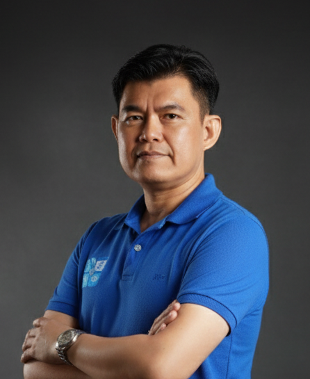
Asst. Prof. Dr. Titipong Kaewlek, Ph.D.
Co-founder of DIP-Lab
Launch Processing Lab
Sign in with your student credentials to access the interactive workstation and process images in real time.
Student Login